QuantLib Architecture and Design Philosophy

QuantLib-Python | QuantLib | 2025.04.12

1️⃣ QuantLib's Object-Oriented Design Principles

QuantLib is a powerful open-source library for financial applications, built on a well-designed object-oriented architecture. This design helps model complex financial concepts clearly and maximizes code reusability and extensibility.

✅ Core Design Principles

QuantLib follows these object-oriented design principles:

Abstraction

Complex financial concepts and products are abstracted into easy-to-understand classes. For example, all financial instruments inherit from the Instrument abstract class. This allows developers to focus on the product's characteristics rather than specific implementation details.

python

# Example of abstraction:
# All financial instruments have NPV (Net Present Value) calculation
instrument = some_financial_instrument

# Same interface regardless of specific implementation
price = instrument.NPV()

Encapsulation

Each class encapsulates its data and functions internally, allowing access only through well-defined interfaces. This increases code stability and minimizes impact when changes are made.

Inheritance

Code reusability is increased by inheriting properties and methods from base classes to derived classes. For example, all option types inherit from the Option class and share common properties and methods.

Polymorphism

Different implementations are supported through the same interface. This allows flexible application of various financial models and methodologies.

python

# Example of polymorphism: 
# Using different pricing engines with the same interface
option.setPricingEngine(analytic_engine)      # Analytical method
option.setPricingEngine(monte_carlo_engine)   # Monte Carlo method
option.setPricingEngine(binomial_tree_engine) # Binomial tree method

✅ Modularity and Extensibility

QuantLib provides extensibility through a modular structure. New financial instruments, models, and algorithms can be easily integrated into the existing framework. This is an important feature for responding to rapid changes and innovations in financial markets.

2️⃣ Main Design Patterns

QuantLib uses several design patterns to manage the complexity of financial applications. Let's look at some of the most important patterns.

✅ Observer/Observable Pattern

Financial market data constantly changes, and changes in one piece of data affect multiple calculations. QuantLib uses the Observer/Observable pattern to manage these dependencies.

Observable: An observable object that sends notifications to all registered Observers when its state changes.
Observer: Observes Observable objects and updates its own state when it receives change notifications.

python

import QuantLib as ql

# SimpleQuote is a type of Observable
spot_price = ql.SimpleQuote(100.0)

# Other objects that depend on this price are registered as Observers
# They automatically update when the price changes

# When value changes, notifications are sent to all dependent objects
spot_price.setValue(105.0)

This pattern is especially useful in financial models. For example, when the underlying asset price changes, all derivative prices that depend on it are automatically updated.

✅ Handle/Quote Pattern

QuantLib uses the Handle/Quote pattern to flexibly manage financial market data.

Quote: Interface representing market data (e.g., stock price, interest rate, volatility)
Handle: Wrapper class that stores references to Quotes, allowing the reference target to be changed at runtime

python

import QuantLib as ql

# Create market data
spot_price = ql.SimpleQuote(100.0)
spot_handle = ql.QuoteHandle(spot_price)

# Create object using handle
process = ql.BlackScholesProcess(spot_handle, ...)

# Later, update underlying data without changing the reference
spot_price.setValue(105.0)  # Automatically reflected in process

This pattern is useful for handling real-time market data updates or applying different market scenarios to the same model.

✅ LazyObject Pattern

Financial calculations are often computationally expensive. QuantLib implements lazy evaluation using the LazyObject pattern, performing calculations only when needed.

LazyObject: Object that delays calculations until actually needed and recalculates only when dependent data changes

python

# YieldTermStructure inherits from LazyObject
# Internal calculations are performed only when interest rates are actually needed
rate = yield_curve.zeroRate(5.0, ql.Continuous)

This pattern is particularly useful for computationally expensive objects like complex yield curves or volatility surfaces.

✅ Factory Pattern

QuantLib uses the factory pattern to manage the creation of various financial objects.

Factory: Encapsulates object creation logic, allowing client code to work with interfaces instead of concrete classes.

python

# Example of option factory 
# (QuantLib doesn't explicitly provide factory classes,
# but many creation patterns follow this concept)
engine = ql.MakeFdBlackScholesVanillaEngine(process)
        .withTGrid(100)
        .withXGrid(100)
        .withCashDividendModel()

3️⃣ Class Hierarchy Overview

QuantLib provides a rich class hierarchy for modeling financial concepts. Let's look at the main hierarchical structures.

✅ Financial Instrument Hierarchy

All financial instruments are derived from the Instrument abstract class:

Instrument
├── Option
│   ├── VanillaOption
│   ├── ExoticOption
│   │   ├── BarrierOption
│   │   ├── AsianOption
│   │   └── ...
│   └── ...
├── Bond
│   ├── ZeroCouponBond
│   ├── FixedRateBond
│   ├── FloatingRateBond
│   └── ...
├── Swap
│   ├── VanillaSwap
│   ├── CrossCurrencySwap
│   └── ...
└── ...

This hierarchy maximizes code reusability by implementing common functionality in parent classes and specific product characteristics in child classes.

✅ Market Data Structure

Market data is organized in the following hierarchy:

TermStructure
├── YieldTermStructure
│   ├── FlatForward
│   ├── PiecewiseYieldCurve
│   └── ...
├── VolatilityTermStructure
│   ├── BlackConstantVol
│   ├── BlackVarianceSurface
│   └── ...
└── DefaultTermStructure
    ├── FlatHazardRate
    ├── PiecewiseDefaultCurve
    └── ...

This structure allows access to various market data through a consistent interface.

✅ Pricing Engines

Pricing engines implement algorithms for calculating financial instrument prices:

PricingEngine
├── VanillaOptionEngine
│   ├── AnalyticEuropeanEngine
│   ├── BinomialVanillaEngine
│   ├── MCEuropeanEngine
│   └── ...
├── BondEngine
│   ├── DiscountingBondEngine
│   └── ...
└── ...

This design allows the same financial instrument to be priced using various methodologies.

4️⃣ Python Binding Features

QuantLib was originally written in C++, but it can also be used in Python through QuantLib-Python. The Python binding has several characteristics.

✅ Interface Through SWIG

QuantLib-Python uses SWIG (Simplified Wrapper and Interface Generator) to wrap C++ code for Python. This exposes C++ classes and functions as Python modules.

✅ Differences Between C++ and Python

The Python interface is almost identical to the C++ library, but there are some differences:

Naming conventions: Some methods in Python follow snake_case instead of C++'s camelCase.
Operator overloading: Some C++ operator overloading is implemented differently in Python.
Memory management: Python's garbage collection manages the lifetime of C++ objects.

✅ Advantages of Using Python

Python is a popular language for financial analysis, and using QuantLib-Python offers the following advantages:

Easy learning curve: Python is easier to learn than C++ and provides more concise syntax.
Data science ecosystem integration: Easy integration with data science libraries like NumPy, pandas, and matplotlib.
Rapid prototyping: Python's fast development speed makes it suitable for quickly prototyping financial models.

python

# Python integration example
import QuantLib as ql
import numpy as np
import pandas as pd
import matplotlib.pyplot as plt

# Perform QuantLib calculations
spot_prices = np.linspace(80, 120, 41)
option_prices = []

for spot in spot_prices:
    # Set underlying asset price
    spot_quote.setValue(spot)
    # Perform calculation, european_option: 
    # object created in previous page example
    option_prices.append(european_option.NPV())

# Result analysis using Pandas and Matplotlib
df = pd.DataFrame({'SpotPrice': spot_prices, 
                   'OptionPrice': option_prices})
plt.figure(figsize=(10, 6))
plt.plot(df['SpotPrice'], df['OptionPrice'])
plt.title('Option Price vs. Spot Price')
plt.xlabel('Spot Price')
plt.ylabel('Option Price')
plt.grid(True)
plt.show()

python

# Result

architecture_option_price

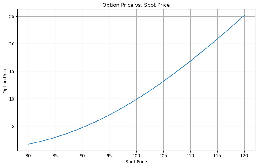
5️⃣ Example: Basic Object Creation and Interaction

To better understand QuantLib's architecture, let's look at the interaction between major objects through a simple example. In this example, we'll implement the basic process of pricing a European call option.

python

import QuantLib as ql

# 1. Date setup
valuation_date = ql.Date(15, 1, 2025)
ql.Settings.instance().evaluationDate = valuation_date
maturity_date = ql.Date(15, 1, 2026)  # 1 year maturity

# 2. Market data setup (Observable objects)
spot_price = ql.SimpleQuote(100.0)      # Underlying asset price
risk_free_rate = ql.SimpleQuote(0.05)   # Risk-free interest rate
volatility = ql.SimpleQuote(0.2)        # Volatility

# 3. Handle creation (interface abstraction)
spot_handle = ql.QuoteHandle(spot_price)
rate_handle = ql.YieldTermStructureHandle(
    ql.FlatForward(valuation_date, 
                   ql.QuoteHandle(risk_free_rate), 
                   ql.Actual365Fixed())
)
vol_handle = ql.BlackVolTermStructureHandle(
    ql.BlackConstantVol(valuation_date, 
                        ql.NullCalendar(), 
                        ql.QuoteHandle(volatility), 
                        ql.Actual365Fixed())
)

# 4. Process creation (stochastic process modeling)
process = ql.BlackScholesProcess(spot_handle, 
                                 rate_handle, 
                                 vol_handle)

# 5. Option setup (product definition)
strike = 100.0
option_type = ql.Option.Call
payoff = ql.PlainVanillaPayoff(option_type, strike)
exercise = ql.EuropeanExercise(maturity_date)
option = ql.VanillaOption(payoff, exercise)

# 6. Pricing engine setup (algorithm selection)
engine = ql.AnalyticEuropeanEngine(process)
option.setPricingEngine(engine)

# 7. Result calculation
option_price = option.NPV()
option_delta = option.delta()
option_gamma = option.gamma()
# QuantLib calculates vega for 1% change
option_vega = option.vega() / 100

print(f"Option price: {option_price:.4f}")
print(f"Delta: {option_delta:.4f}")
print(f"Gamma: {option_gamma:.6f}")
print(f"Vega: {option_vega:.4f}")

# 8. Market data change (Observer/Observable pattern demonstration)
print("\nChanging underlying asset price to 110:")

# This change is automatically propagated to all dependent objects
spot_price.setValue(110.0)  

# Result recalculation 
# (lazy evaluation - calculated only when needed)
print(f"Option price: {option.NPV():.4f}")
print(f"Delta: {option.delta():.4f}")

python

# Output
# Option price: 10.4506
# Delta: 0.6368
# Gamma: 0.018762
# Vega: 0.3752

# Changing underlying asset price to 110:
# Option price: 17.6630
# Delta: 0.7958

This example demonstrates QuantLib's key architectural features:

Object-oriented design: Each financial concept (dates, market data, instruments, engines) is modeled as independent classes.
Observer/Observable pattern: Market data changes are automatically propagated to all dependent objects.
Handle/Quote pattern: References to market data are abstracted.
Lazy evaluation: Results are calculated only when needed.

6️⃣ Practical Application: Comparing Different Pricing Methods

In financial modeling, it's common to price the same instrument using multiple methods. QuantLib's flexible architecture makes this easy to implement.

python

import QuantLib as ql
import matplotlib.pyplot as plt
import numpy as np
import time

# Basic setup (same as previous example)
valuation_date = ql.Date(15, 1, 2025)
ql.Settings.instance().evaluationDate = valuation_date
maturity_date = ql.Date(15, 1, 2026)
spot = ql.SimpleQuote(100.0)
rate = ql.SimpleQuote(0.05)
vol = ql.SimpleQuote(0.2)

spot_handle = ql.QuoteHandle(spot)
rate_handle = ql.YieldTermStructureHandle(
    ql.FlatForward(valuation_date, 
                   ql.QuoteHandle(rate), 
                   ql.Actual365Fixed())
)
vol_handle = ql.BlackVolTermStructureHandle(
    ql.BlackConstantVol(valuation_date, 
                        ql.NullCalendar(), 
                        ql.QuoteHandle(vol), 
                        ql.Actual365Fixed())
)

process = ql.BlackScholesProcess(spot_handle, 
                                 rate_handle, 
                                 vol_handle)

# Option setup
strike = 100.0
option_type = ql.Option.Call
payoff = ql.PlainVanillaPayoff(option_type, strike)
exercise = ql.EuropeanExercise(maturity_date)
option = ql.VanillaOption(payoff, exercise)

# Setup various pricing engines
# 1. Analytical method (Black-Scholes formula)
analytic_engine = ql.AnalyticEuropeanEngine(process)

# 2. Binomial tree method (Cox-Ross-Rubinstein model)
binomial_engine = ql.BinomialVanillaEngine(process, "crr", 100)

# 3. Monte Carlo simulation method
mc_engine = ql.MCEuropeanEngine(process, "pseudorandom", 
                                timeSteps=100, 
                                requiredSamples=10000,
                                seed=42)

# Calculate prices and measure performance for each method
engines = [
    ("Black-Scholes Analytical Method", analytic_engine),
    ("Binomial Tree Method (100 Steps)", binomial_engine),
    ("Monte Carlo Method (10,000 samples)", mc_engine)
]

results = []

for name, engine in engines:
    start_time = time.time()
    option.setPricingEngine(engine)
    price = option.NPV()
    elapsed_time = time.time() - start_time
    results.append({
        "Method": name,
        "Price": price,
        "Time (seconds)": elapsed_time
    })

# Output results
print("Comparison of different pricing methods:")
for result in results:
    print(f"{result['Method']}: {result['Price']:.6f} (Time: {result['Time (seconds)']:.6f}s)")

# Compare results for different strike prices
strikes = np.linspace(80, 120, 21)
prices = {name: [] for name, _ in engines}

for strike in strikes:
    payoff = ql.PlainVanillaPayoff(option_type, strike)
    option = ql.VanillaOption(payoff, exercise)
    
    for name, engine in engines:
        option.setPricingEngine(engine)
        prices[name].append(option.NPV())

# Visualize results
plt.figure(figsize=(10, 6))
for name, _ in engines:
    plt.plot(strikes, prices[name], label=name)
    
plt.title('Option Price by Strike Price')
plt.xlabel('Strike Price')
plt.ylabel('Option Price')
plt.legend()
plt.grid(True)
plt.show()

python

# Output
# Comparison of different pricing methods:
# Black-Scholes Analytical Method: 10.450584 (Time: 0.000141s)
# Binomial Tree Method (100 Steps): 10.429986 (Time: 0.000076s)
# Monte Carlo Method (10,000 samples): 10.526726 (Time: 0.166369s)

architecture_option_price

This example shows how flexible QuantLib's architecture is. The same option can be priced using various methodologies, and you can compare the results and performance of each method.

7️⃣ Summary and Next Steps

In this section, we explored QuantLib's architecture and design philosophy. QuantLib follows object-oriented design principles and uses design patterns like Observer/Observable, Handle/Quote, and LazyObject to manage the complexity of financial applications. This architecture increases code reusability, extensibility, and maintainability, allowing various financial instruments and models to be implemented in a consistent manner.

Through Python bindings, QuantLib's powerful features can be easily integrated with data science libraries like NumPy, pandas, and matplotlib, making financial analysis and modeling work more efficient.

Additional Learning Resources

"Implementing QuantLib" by Luigi Ballabio (QuantLib's main developer)
"C++ Design Patterns and Derivatives Pricing" by Mark S. Joshi
QuantLib Official Documentation
QuantLib GitHub Repository

QuantLib Architecture and Design Philosophy ​

1️⃣ QuantLib's Object-Oriented Design Principles ​

✅ Core Design Principles ​

✅ Modularity and Extensibility ​

2️⃣ Main Design Patterns ​

✅ Observer/Observable Pattern ​

✅ Handle/Quote Pattern ​

✅ LazyObject Pattern ​

✅ Factory Pattern ​

3️⃣ Class Hierarchy Overview ​

✅ Financial Instrument Hierarchy ​

✅ Market Data Structure ​

✅ Pricing Engines ​

4️⃣ Python Binding Features ​

✅ Interface Through SWIG ​

✅ Differences Between C++ and Python ​

✅ Advantages of Using Python ​

5️⃣ Example: Basic Object Creation and Interaction ​

6️⃣ Practical Application: Comparing Different Pricing Methods ​

7️⃣ Summary and Next Steps ​

Additional Learning Resources ​

QuantLib Architecture and Design Philosophy

1️⃣ QuantLib's Object-Oriented Design Principles

✅ Core Design Principles

✅ Modularity and Extensibility

2️⃣ Main Design Patterns

✅ Observer/Observable Pattern

✅ Handle/Quote Pattern

✅ LazyObject Pattern

✅ Factory Pattern

3️⃣ Class Hierarchy Overview

✅ Financial Instrument Hierarchy

✅ Market Data Structure

✅ Pricing Engines

4️⃣ Python Binding Features

✅ Interface Through SWIG

✅ Differences Between C++ and Python

✅ Advantages of Using Python

5️⃣ Example: Basic Object Creation and Interaction

6️⃣ Practical Application: Comparing Different Pricing Methods

7️⃣ Summary and Next Steps

Additional Learning Resources